From logic gates to a programming language using the Hex architecture

This note walks through a hardware implementation of a simple processor and complete compiler for a programming language targeted at it. The processor architecture is designed to as simple as possible but provide a sensible target for the compilation of complex programs using simple strategies. The implementation of the processor and its supporting tooling is small and self contained so to be understandable and easily extendable. Besides being an interesting side project, my motivation was to create a complete example as a point of reference to explain how programming languages work and correspond to the underlying hardware of a computer processor, or to provide a useful reference for compilers and simulators, a starting point for another project or just a curiosity in itself.

First, to provide some background. The project is based on the Hex processor architecture that was designed by David May as a vehicle for teaching about how computers work at the University of Bristol, whilst being flexible enough to execute substantial programs and easily extensible. David provided a simulator written in C and a bootstrapping compiler written in an accompanying simple imperative programming language called X. The design of Hex draws on the Transputer architecture and the earlier Simple 42, particularly with the use of short instruction encodings, a prefixing mechanism for creating larger immediates and A, B and C registers for expression evaluation. These kind of architectural features made the silicon implementation of the Simple 42 and Transputers small enough to fit on a single chip in the technology of the day. X draws on the basic sequential features of the occam programming language but it not dissimilar to a small subset of C, for example. I include some more historical details at the end.

In my implementation, I have created a simple C++ toolchain with a simulator, Hex assembler and X language compiler, and a Verilog implementation of Hex. Before describing them, the next two sections introduce Hex and X.

Table of contents

1. The Hex architecture
2. The X language
3. Hex processor integrated circuit
4. Hex tooling
5. A historical note
6. Summary
7. Similar projects
8. Further reading

The Hex architecture

The Hex architecture is described in detail in a separate PDF, but I will give a brief summary here and focus on several important aspects for reference. Hex has four registers: program counter pc, operand register oreg and the A and B registers areg and breg used for expression evaluation. The architecture is agnostic of a particular word size, but it has to be a minimum of a byte and multiples of a byte. In the included implementation the word size is 4 bytes. Hex has sixteen instructions (hence its name!) that are summarised in the following table. Each instruction has a 4-bit opcode and a 4-bit immediate. The immediate value can be extended using the prefix instructions to form a wider value in the oreg, adding four bits per instruction. Operations beyond the 16 available encodings are made accessible by the OPR instruction that encodes the operation type with its immediate. The instructions are grouped into memory access with absolute or relative addressing modes, loading of constants, branching, inter-register operations and supervisor calls.

Prefixing

Prefixing using the PFIX and NFIX operations generates operand values in oreg larger than the 4-bit instruction immediate. For example, the following instructions generate the value 16 in oreg and use LDAC to assign it to areg :

PFIX 1  # oreg = oreg (1) << 4 (0x000010)
LDAC 0  # areg = oreg 16

Prefixes can be chained to extend the operand range, for example, generating the value 496 requires two positive prefixes before a load constant instruction:

PFIX 1  # oreg = oreg (1) << 4 (0x000010)
PFIX 15 # oreg = oreg (31) << 4 (0x0001f0)
LDAC 0  # areg = oreg 496

Negative values always require a negative prefix to fill the top most oreg bits with ones, so to load the value -1 into oreg then areg:

NFIX 15 # oreg = 0xFFFFFF00 | oreg (15) << 4 (0xfffffff0)
LDAC 15 # areg = oreg 4294967295

And to load -512, a positive prefix is required to scale the negative value:

NFIX 14 # oreg = 0xFFFFFF00 | oreg (14) << 4 (0xffffffe0)
PFIX 0  # oreg = oreg (4294967264) << 4 (0xfffffe00)
LDAC 0  # areg = oreg 4294966784

Inter-register operations

The inter-register operations use the OPR opcode and consist only of addition and subtraction. The group can be extended by implementing additional immediate opcodes to add new operations to the processor (such as other arithmetic and bitwise operations). The 4-bit immediate supports up to 16 inter-register operations without the need for prefixing, but many more with prefixing and the according overhead to form larger immediates. The following instruction sequence adds two numbers from fixed locations in memory, with the result written to areg:

LDAM 1  # areg = mem[oreg (0x000001)] (7)
LDBM 2  # breg = mem[oreg (0x000002)] (9)
OPR  1  # ADD areg = areg (7) + breg (9) (16)

A special inter-register operation is a supervisor call that transfers control to the system to complete an action such as read or write from a file, or to halt the program. The supervisor call type is encoded in the oreg and arguments and return values specific to the call type are passed and returned on the stack using the standard calling convention. An example code sequence to invoke the exit supervisor call is:

LDAC 0  # Set areg to 0, the exit opcode value.
LDBM 1  # Load the stack pointer in breg.
STAI 2  # Store areg into stack offset two as a parameter.
LDAC 0  # Load the exit opcode.
OPR SVC # Perform the supervisor call

With the following execution trace, noting that the simulator implements the system call directly rather than being handled by a kernel routine:

LDAC 0  # areg = oreg 0
LDBM 1  # breg = mem[oreg (0x000001)] (16383)
STAI 2  # mem[breg (16383) + oreg (2) = 0x004001] = areg (0)
LDAC 0  # areg = oreg 0
OPR  3  # exit 0

Load-store operations

There are two variants of load and store instructions: using absolute addresses and addresses relative to a base address. Absolute addressing (LDAM, LDBM and STAM) is intended to access objects in memory that are allocated at offsets that are fixed with respect to a program, such as constant values and global variables. Relative-addressing (LDAI, LDBI and STAI) is typically used to access objects that are relative to a dynamic position, such as the stack pointer, or index into an array. The particular variants of load/store instructions is influenced by their targeting from a compiler. Having pairs of load instructions that can write to areg or breg (such as LDAM and LDBM) gives flexibility when generating operands for binary operations, whereas having only single variants of stores (STAM and STAI) fits most cases where expression results generated into areg need to be written to memory.

Branching

For branching, a relative branch is provided with BR, which can be used, for example, to reach a label location. Conditional branch versions BRZ and BRN are used to implement logical binary operations (less than, equal etc) and BRB is an absolute branch that is used, for example, to return to a calling function using an address retrieved from memory (see example in next section).

Address generation

A special constant-loading instruction LDAP is used to generate bytewise program addresses, relative to the program counter, such as for branch targets. The following instruction sequence performs a call to foo but first loads the return (link) address using LDAP to use with BR. The callee foo returns to the caller using BRB.

FUNC foo
LDBM 1
STAI 0 # Save caller address
...
LDBI 0 # Restore caller address
OPR 0  # Return to caller

PROC main
...
LDAP lab2
BR foo
lab2

These instructions have the following execution trace:

main+32  LDAP 2   # areg = pc (60) + oreg (2) 62
main+33  NFIX 13  # oreg = 0xFFFFFF00 | oreg (13) << 4 (0xffffffd0)
main+34  BR   1   # pc = pc + oreg (4294967249) (0x00000f)
foo+0    LDBM 1   # breg = mem[oreg (0x000001)] (199994)
foo+1    STAI 0   # mem[breg (199994) + oreg (0) = 0x030d3a] = areg (62)
...
foo+10   LDBI 0   # breg = mem[breg (199994) + oreg (0) = 0x030d3a] (62)
foo+11   OPR  0   # BRB pc = breg (0x00003e)
main+35  ...

The X language

The X language is defined in a separate PDF. X is simple enough that it can be compiled using simple techniques to the Hex architecture, whilst providing enough flexibility to express complex programs such as its own compiler (more on that later). X is an imperative language and has features for procedure calling, composition of statements, looping and conditional statements, expressions including function calls, and representation of memory with variables and arrays. To give an indicative example of X programming, the following program implements Bubblesort to sort an array of four elements:

val length = 4;
var data[length];

proc sort(array a, val n) is
  var i;
  var j;
  var tmp;
{ i := 0;
  while i < n do
  { j := 0
  ; while j < n - i - 1 do
    { if a[j] > a[j+1] then
      { tmp := a[j]
      ; a[j] := a[j+1]
      ; a[j+1] := tmp
      }
      else skip
    ; j := j + 1
    }
  ; i := i + 1
  }
}

proc main() is
{ data[0] := 3
; data[1] := 2
; data[2] := 1
; data[3] := 0
; sort(data, length)
}

Limitations of X to note that simplify its implementation are:

• Arrays are limited to one dimension.

• No operator precedence to avoid built-in rules so precedence must be indicated explicitly with bracketing (apart from associative operators).

• Conditional statements (beginning if) must always have an else part to simplify parsing.

• Variables can only be passed by value into procedures.

• There is no block scoping so variable and array declarations can only be made at global and procedure scopes. Similarly, nested definitions of procedures are not permitted.

Other noteworthy features of X are:

• There are two types of procedure: processes (using the proc keyword) that execute a sequence of steps with possible side effects, and functions (using the funckeyword ) that have no side effects and return a value.

• Names in a program are introduced as definitions of processes or functions, declarations that represent memory locations, and abbreviations that introduce alternative names for expressions, arrays, processes and functions.

• The scoping and abbreviation rules are defined so that that actual parameters act as abbreviations of the supplied formals. This allows processes and functions to be compiled by either as closed subroutines or by substitution of the body at the call site, either as a source code transformation or compiler optimisation. For example, given the definition proc foo(val a, array b) is B, it can be called as a subroutine: foo(x, y) or substituted: val a = x; array b = y; B providing the names are unique in the procedure.

• A valof element allows processes to be called from expressions to generate values, however it is not implemented in xhexb or xcmp.

Hex processor integrated circuit

A hardware implementation of the Hex processor is written in System Verilog, processor.sv, in just 150 lines. This implementation is single cycle in that all elements of instruction execution (ie instruction fetch from memory, decode, instruction memory access and state writeback) are completed in that time. A separate memory module, memory.sv implements a single-cycle random-access memory with two ports: one for instruction fetch and the other for data access so that they can occur simultaneously in the same cycle. Note that because memory access time increases with the memory capacity, a implementation of Hex accessing a large memory (ie more than a few thousand bytes) would add pipelining to hide the latency to memory. Some degree of pipelining is standard in processor implementations. The hardware design is simulated using Verilator, with C++ testbench driver code in hextb.cpp.

Using OpenROAD, an open-source tool chain for performing synthesis, optimisation and physical layout of digital circuits, we can compile Hex into an integrated circuit layout in order that it could be manufactured into a silicon device. OpenROAD uses the SkyWater Process Design Kit (PDK), for creating designs in 130 nm process technology, which was a technology first commercialised in 2001. The PDK is a collection of analog and digital cell libraries, design rules and tooling. Since OpenROAD uses Yosys for synthesis, and it doesn’t support particular SystemVerilog features, I used sv2v to convert the implementation to plain Verilog 2005 (see processor.v).

The physical design is based on an OpenROAD default flow, which takes a few minutes to be compiled from the source RTL. The final design has the following characteristics:

• A die size of ~280x280 microns.
• A total of 9,719 standard cells.
• A cell area of 16,706 square microns at 25% utilisation.
• A clock speed of 229 MHz.
• Total switching power of 4.12 mW.

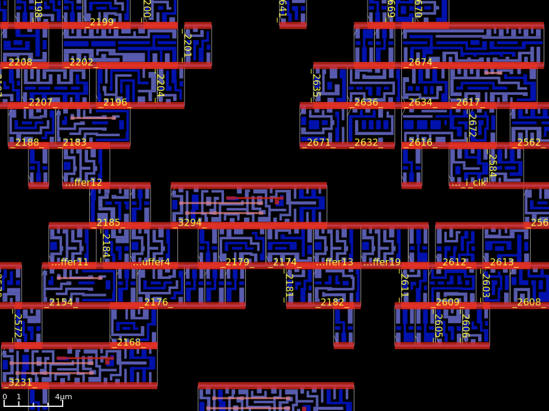
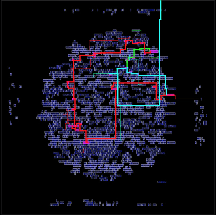
The OpenROAD GUI provides many ways to visualise and explore the design. The following images are some examples of the different views.

Hex tooling

There are three tools provided in the Hex toolchain: a Hex instruction set simulator hexsim, a Hex assembler hexasm and an X compiler xcmp. Instructions on how to build the tools are included in the documentation. The implementation is provided in a small number of source files (with only one external dependency on boost::format):

• General Hex definitions are provided in hex.hpp and hex.cpp.

• The Hex simulator is implemented in the headers hexsim.hpp and hexsimio.hpp. (Note that listings for a complete simulator in C are given in the Hex definition (PDF).)

• The Hex assembler is implemented in the header hexasm.hpp.

• The X compiler is implemented in the header xcmp.hpp.

• Driver code for the respective command-line tools hexsim, hexasm and xcmp is implemented in hexsim.cpp, hexasm.cpp and xcmp.cpp.

A simple example

Taking a most basic example of an assembly program that simply exits:

➜ cat tests/asm/exit0.S
BR start
DATA 16383 # sp
start
LDAC 0 # areg <- 0
LDBM 1 # breg <- sp
STAI 2 # sp[2] <- areg
LDAC 0
OPR SVC

The assembler can display the program layout in memory and computed symbol values:

➜ hexasm tests/asm/exit0.S --instrs
00000000 BR start (7)         (1 bytes)
0x000004 DATA 16383           (4 bytes)
0x000008 start                (0 bytes)
0x000008 LDAC 0               (1 bytes)
0x000009 LDBM 1               (1 bytes)
0x00000a STAI 2               (1 bytes)
0x00000b LDAC 0               (1 bytes)
0x00000c OPR SVC              (1 bytes)
00000000 PADDING 3            (3 bytes)
13 bytes

And create a 13-byte executable binary:

➜ hexasm tests/asm/exit0.S

This binary can then be simulated with tracing to show what’s going on (the first column is the cycle count and the second is the pc value):

➜ hexsim a.out -t
0      0      BR   7  pc = pc + oreg (7) (0x000008)
1      8      LDAC 0  areg = oreg 0
2      9      LDBM 1  breg = mem[oreg (0x000001)] (16383)
3      10     STAI 2  mem[breg (16383) + oreg (2) = 0x004001] = areg (0)
4      11     LDAC 0  areg = oreg 0
5      12     OPR  3  exit 0

The X compiler can be used to produce more complex Hex programs. Starting with a similar most basic program written in X:

proc main() is skip

This null program is compiled into Hex assembly, where the entry code calls main then exits, and main does nothing (apart from saving and restoring the link location):

➜ xcmp tests/x/exit.x --insts-lowered
BR start
DATA 199999
start
LDAP _exit
BR main
_exit
LDBM 1
LDAC 0
STAI 2
OPR SVC

PROC main
LDBM 1
STAI 0
lab0
LDBM 1
LDBI 0
OPR BRB

And when simulated produces the following trace where execution through main can be seen since it is the only labelled portion of the code:

➜ hexsim a.out -t
0      0                   BR   7  pc = pc + oreg (7) (0x000008)
1      8                   LDAP 1  areg = pc (9) + oreg (1) 10
2      9                   BR   4  pc = pc + oreg (4) (0x00000e)
3      14     main+0       LDBM 1  breg = mem[oreg (0x000001)] (199999)
4      15     main+1       STAI 0  mem[breg (199999) + oreg (0) = 0x030d3f] = areg (10)
5      16     main+2       LDBM 1  breg = mem[oreg (0x000001)] (199999)
6      17     main+3       LDBI 0  breg = mem[breg (199999) + oreg (0) = 0x030d3f] (10)
7      18     main+4       OPR  0  BRB pc = breg (0x00000a)
8      10                  LDBM 1  breg = mem[oreg (0x000001)] (199999)
9      11                  LDAC 0  areg = oreg 0
10     12                  STAI 2  mem[breg (199999) + oreg (2) = 0x030d41] = areg (0)
11     13                  OPR  3  exit 0

The program can also be run on the Verilog Hex implementation using hextb (which doesn’t provide as rich instruction tracing as hexsim):

➜ hextb a.out -t
Wrote 20 bytes to memory
[11] 8      0x51 LDAP
[13] 9      0x94 BR
[15] 14     0x11 LDBM
[17] 15     0x80 STAI
[19] 16     0x11 LDBM
[21] 17     0x70 LDBI
[23] 18     0xd0 OPR
[25] 10     0x11 LDBM
[27] 11     0x30 LDAC
[29] 12     0x82 STAI
[31] 13     0xd3 OPR
exit 0

Hello World

A more fulsome example is ‘Hello World’, where the main process is simply:

proc main() is prints("hello world\n")

And prints unpacks the bytewise string representation by using routines for performing division and remainder by 265. The full program listing is:

➜ cat tests/x/hello_prints.x
val put = 1;
val bytesperword = 4;
var div_x;

proc main() is prints("hello world\n")

proc putval(val c) is put(c, 0)

func lsu(val x, val y) is
  if (x < 0) = (y < 0)
  then
    return x < y
  else
    return y < 0

func div_step(val b, val y) is
  var r;
{ if (y < 0) or (~lsu(y, div_x))
  then
    r := 0
  else
    r := div_step(b + b, y + y);
  if ~lsu(div_x, y)
  then
  { div_x := div_x - y;
    r := r + b
  }
  else
    skip;
  return r
}

func div(val n, val m) is
{ div_x := n;
  if lsu(n, m)
  then
    return 0
  else
    return div_step(1, m)
}

func rem(val n, val m) is
  var x;
{ x := div(n, m);
  return div_x
}

proc prints(array s) is
  var n;
  var p;
  var w;
  var l;
  var b;
{ n := 1;
  p := 0;
  w := s[p];
  l := rem(w, 256);
  w := div(w, 256);
  b := 1;
  while (n <= l) do
  { putval(rem(w, 256));
    w := div(w, 256);
    n := n + 1;
    b := b + 1;
    if (b = bytesperword)
    then
    { b := 0;
      p := p + 1;
      w := s[p]
    }
    else skip
  }
}

Compiling and running this shows that it takes ~50K cycles to execute and inspecting the trace is clear to see that most time is spent in the arithmetic routines.

➜ xcmp tests/x/hello_prints.x
➜ hexsim a.out
hello world
➜ hexsim a.out -t
...
48902  61                  OPR  3  exit 0

Building an X compiler and bootstrapping

A third example is a complete compiler for X, written in X: xhexb.x written by David May in ~3,000 lines of X. This serves as a challenging program to compile, and interesting that it can bootstrap itself. Using the notation X(Y) to mean compile source Y using binary X, we can first create an xhexb binary by running xcmp(xhexb.x):

➜ xcmp -S tests/x/xhexb.x
...
20739 bytes

We can then use xcmp(xhexb.x) to compile Hello World as xcmp(xhexb.x)(hello_prints.x):

# Create an xhexb compiler binary.
➜ xcmp tests/x/xhexb.x

# Compile Hello World.
➜ hexsim a.out < tests/x/hello_prints.x
tree size: 602
program size: 414
size: 414

# Run it.
➜ hexsim simout2
hello world

Similarly, we can use xcmp(xhexb.x) to bootstrap itself by running xcmp(xhexb.x)(xhexb.x):

# Create an xhexb compiler binary.
➜ xcmp tests/x/xhexb.x

# Use xhexb binary to compile xhexb.x.
➜ hexsim a.out < tests/x/xhexb.x
tree size: 18631
program size: 17093
size: 177097

# Use the bootstrapped xhexb binary to compile Hello World.
➜ hexsim simout2 < tests/x/hello_prints.x
tree size: 602
program size: 414
size: 414

# Run it.
➜ hexsim simout2
hello world

Implementation details

Both the assembler and compiler are based on the xhexb.x bootstrapping compiler for X discussed above.

The assembler works in two main phases:

• Parsing the program to form a list of directives (instructions, labels, data etc).
• Code generation to iterate through the directives and emit binary output.

Before emission, the value of labels must be determined, which involves solving two problems. The first is that for a given relative reference, the length of the encoding (ie number of prefixes) depends on the value of the reference and vice versa. This is solved by iteratively increasing the encoding length until it meets the required range (see instrLen()). The second problem is that the value of a relative reference depends on the length of any relative encodings contained within the range. This is solved by iteratively updating label values until they reach a stable state (see resolveLabels()). The assembler adds additional rudimentary debug information to the binary, with a mapping of instruction ranges to symbol values. This allows the simulator to display the current symbol and offset.

The compiler works a traditional way, structured as a sequence of phases, first creating a parse tree, then performing passes on the tree to optimise it and then lowering the tree to machine instructions:

• Parse the program to form an abstract syntax tree.
• Walk the tree to populate a symbol table with names occurring in the program.
• Walk the tree to propagate constant values within expressions.
• Walk the tree to transform expressions into a canonical form.
• Walk the tree to generate a sequence of intermediate machine instructions.
• Lower the intermediate instructions to machine instructions.
• Optimise the machine instruction sequence.
• Assemble and emit the machine instruction sequence.

Command line options such as --tree are available to inspect the internal representation of the program in between these stages.

Compared with a more sophisticated compiler, Hex and X afford two significant simplifications. First, the small set of features in X make it straightforward to map to directly to machine instructions rather than an intermediate machine-independent representation. Secondly, the register architecture of Hex means that allocation of registers can be handled easily during mapping to machine instructions, rather than having to allocate physical registers to a virtual set as is typical in machines with more registers.

More details of the xhexb compiler implementation are included in the X and Hex notes PDF, with aspects such as the calling convention, handling of operators and arithmetic and memory layout being shared in xcmp.

A historical note

Hex, apart from being related to the Transputer, has some other interesting historical roots. David May learned about languages and compilers from Martin Richards who was a young lecturer when David completed his final-year Computer Science course as a student at King’s College Cambridge (the first student to do so). Martin was the designer of the influential language BCPL and its portable compiler technology. BCPL found its way to Bell Labs where UNIX was being developed. BCPL was the direct precursor to C and so led to the portability of UNIX.

When David moved from Cambridge to Warwick, the only useful language on the Modular One minicomputer that was available was BCPL but the compiler was incomplete. So David completed the compiler and ported BCPL to other computers, including some microprocessors. Using techniques similar to BCPL’s bootstrapping compiler and interpreter, David designed and implemented a concurrent language (EPL), bringing him into contact with Tony Hoare and Iann Barron (founder of the company that designed the Modular One and also of Inmos).

David employed the same techniques again at Inmos to build the first implementation of Occam in the 1980s and then again in 2008 for the project that led to the founding of XMOS (incidentally, I used this compiler in my PhD work to demonstrate techniques of compiling message-passing programs). Hex and X follow directly from the BCPL-derived approaches, used by David as a tool to teach students about instruction sets, compilers, bootstrapping etc.

Summary

Modern processors, languages, compilers, and tooling are complex and difficult to understand. This note walks through possibly the simplest processor architecture that allows a compact implementation of rudimentary tooling and a complete high-level programming language to be targeted at it. The definitions and implementations are contained in a single repository and just a small set of source files, making it an excellent project to use to explore processors and compilers.

Similar projects

The following are some similar projects that include simple implementations of processor toolchains.

• VSPL, is a very simple programming language designed by Martin Richards to be used as a case study for comparing compiler implementations. The provided source distribution includes several implementations of VSPL in different languages.

• Experiments in Computer System Design is a walk through of an implementation of a Tiny Register Machine (TRM) in Verilog with serial communication, DRAM access and multiprocessing (Niklaus Wirth, 2010).

• Selfie is an educational platform for teaching programming languages and runtime systems. It is based on a simplified RISC-V architecture and includes a self-contained self-hosting compiler for a subset of C, an emulator, a hypervisor and a small standard library for the language. These tools are implemented in a single file (~12K lines of code).

• Luz CPU, a simulator, assembler and linker for the Luz processor architecture written by Eli Bendersky.

• Nibbler 4 Bit CPU is a complete description of a processor that has been implemented in discreet logic chips.

• Discrete logic IC CPU us an architecture, discrete-logic implementation and basic tooling including a programming language.

Further reading

• Processor Design: An Introduction a ground-up explanation of how processors work.

• LLVM Kaleidoscope Tutorial which walks through an implementation of a simple programming language using LLVM as a backend for code generation and just-in-time compilation.